Chapter 02 : 1-Dimensional Motion |
Overview | |
Iterative Process: [measure] ➔ [model] ➔ [predict] ➔ ... (repeat) Most of the course can be condensed into a single general equation: Newton's Law:
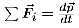
but we don't usually start there. By the end of the course we'll expand into several pages of equations, but by then it's useful to remember where it all starts. |
Tacoma Narrows Bridge (1940)
|
Level of Detail : the 'point mass' model | |
|
|
|
|
Reference Frames | |
Coordinate system used can affect the results of a measurement.
Any fixed or moving coordinate system is fine as long as no acceleration is involved.
We will see later that rotation itself creates an acceleration. |
|
|
|
The Earth is rotating, so technically is not a 'good' reference frame but we routinely use it anyway.
Ball Drop
Do we need to worry about that??? |
Burj Khalifa (Dubai; 828 meters) |
Ball Drop 'Experiment' | |
Drop a ball from about 4 feet (1.22 m) above the floor. Coordinate System Choice:
Record this 'x' coordinate as a function of time.
|
|
How far did the ball travel?
Displacement definition: Δx = x(t2)-x(t1)
Distance \[ s = \int_{t_1}^{t_2}ds \] (zero or positive; can't be negative) (Basically the odometer in your car: continuously accumulating)
|
POSITION : x(t)
|
How fast is the ball moving?
What about speed? Ambiguous...
(A word best not used...)
|
VELOCITY : v(t) = dx/dt
|
Acceleration : rate of change of velocity
Note that for the ball (except for the momentary collision with the floor), a=-9.8 m/s2 |
ACCELERATION : a(t) = dv/dt
|
Can keep going: jerk is defined as da/dt, etc... |
Example : Car Acceleration | |
My 2008 truck took 20 seconds to accelerate from 20 mph to 60 mph.
Assuming the acceleration was constant:
|
![]() |
Motion with Constant Acceleration | |
a=dv/dt so if 'a' is constant what does the graph of v(t) have to look like?
v(t) = vo+at
(our first EQUATION OF MOTION)
Another we can pick off this graph: The average velocity between t=0 and some time t: \[ v_{avg} = \frac{1}{2} ( v_o + v ) \] but since v(t) = vo+at we can also write this as: \[ v_{avg} = v_o + \frac{1}{2} at \] |
|
Position Equation of Motion | |
\[ v_{avg} = v_o + \frac{1}{2} at \] \[ \Delta x = v_{avg} \Delta t \] Making that substitution: \[ x - x_o = ( v_o + \frac{1}{2}at ) t \] Leading to: \[ x = x_o + v_o t + \frac{1}{2}at^2 \]
What is the position equation of motion for the truck? x(t)=? |
|
One Last Useful Equation | |
Everything above involved the time variable, but with the right algebraic steps, we can eliminate time: vavg = Δx/Δt so Δx=vavgt but: vavg = ( vo + v )/2 v = vo+at so t = ( v - vo )/a Making those substitutions, Δx=vavgt becomes: \[ \Delta x = ( \frac{ v+v_o }{2} )( \frac{ v-v_o }{a} ) \] Expanding and rearranging: \[ v^2 = v^2_o + 2 a \Delta x \] As a check, recompute the truck's acceleration using the starting and ending velocities and the distance travelled:
|
|
Putting it All Together | |
A particular high performance car accelerates from rest to 60 MPH in 2.0 sec. It continues at that velocity along a straight road for 8 sec, then slams on the brakes, bringing the car to a stop in 30 meters.
(a) What was the car's average velocity over this entire interval from start to stop? |
Sketch of v(t)
|