Pendulums : Another Type of Periodic Motion

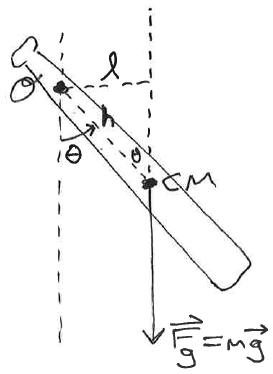
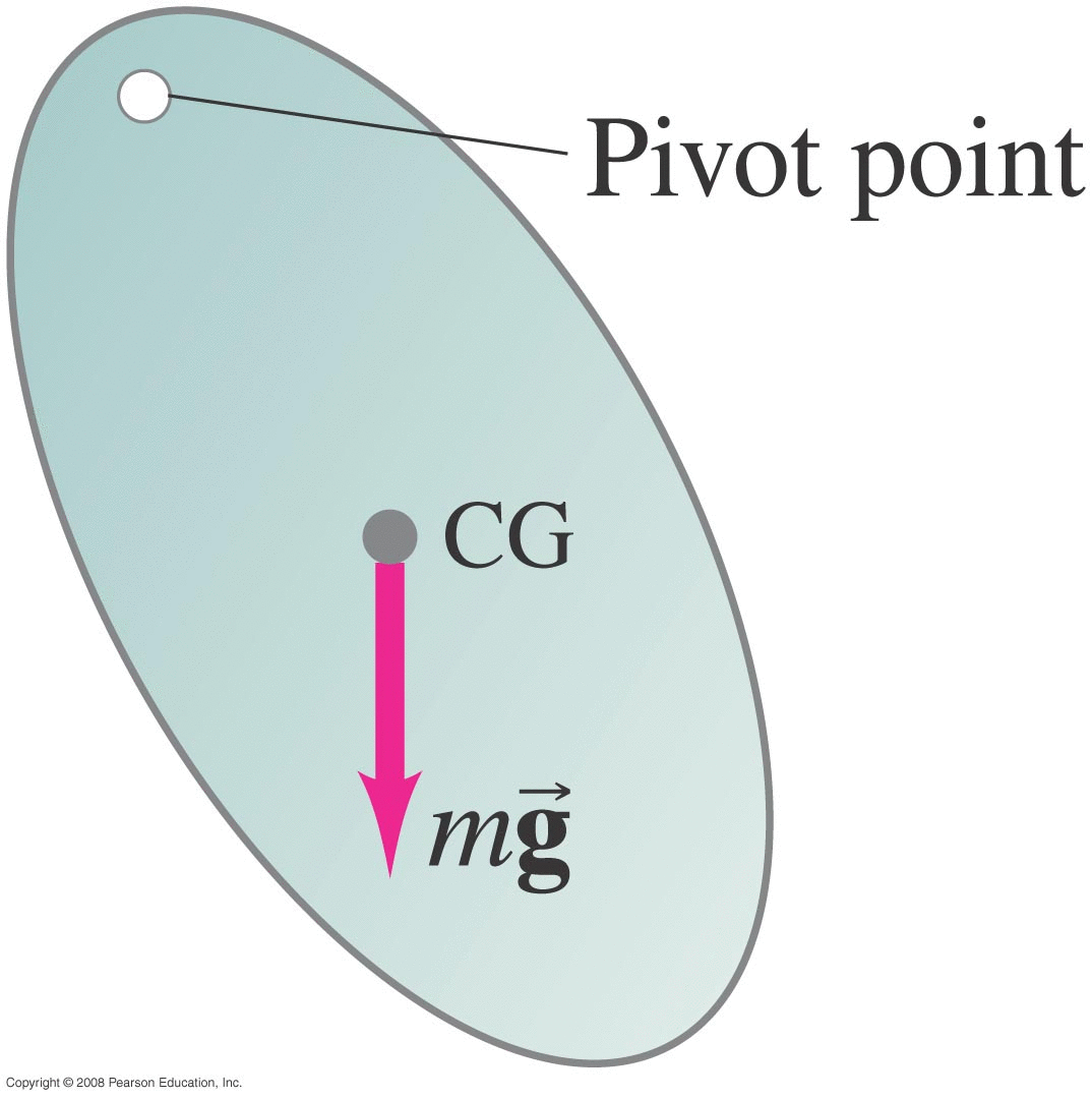
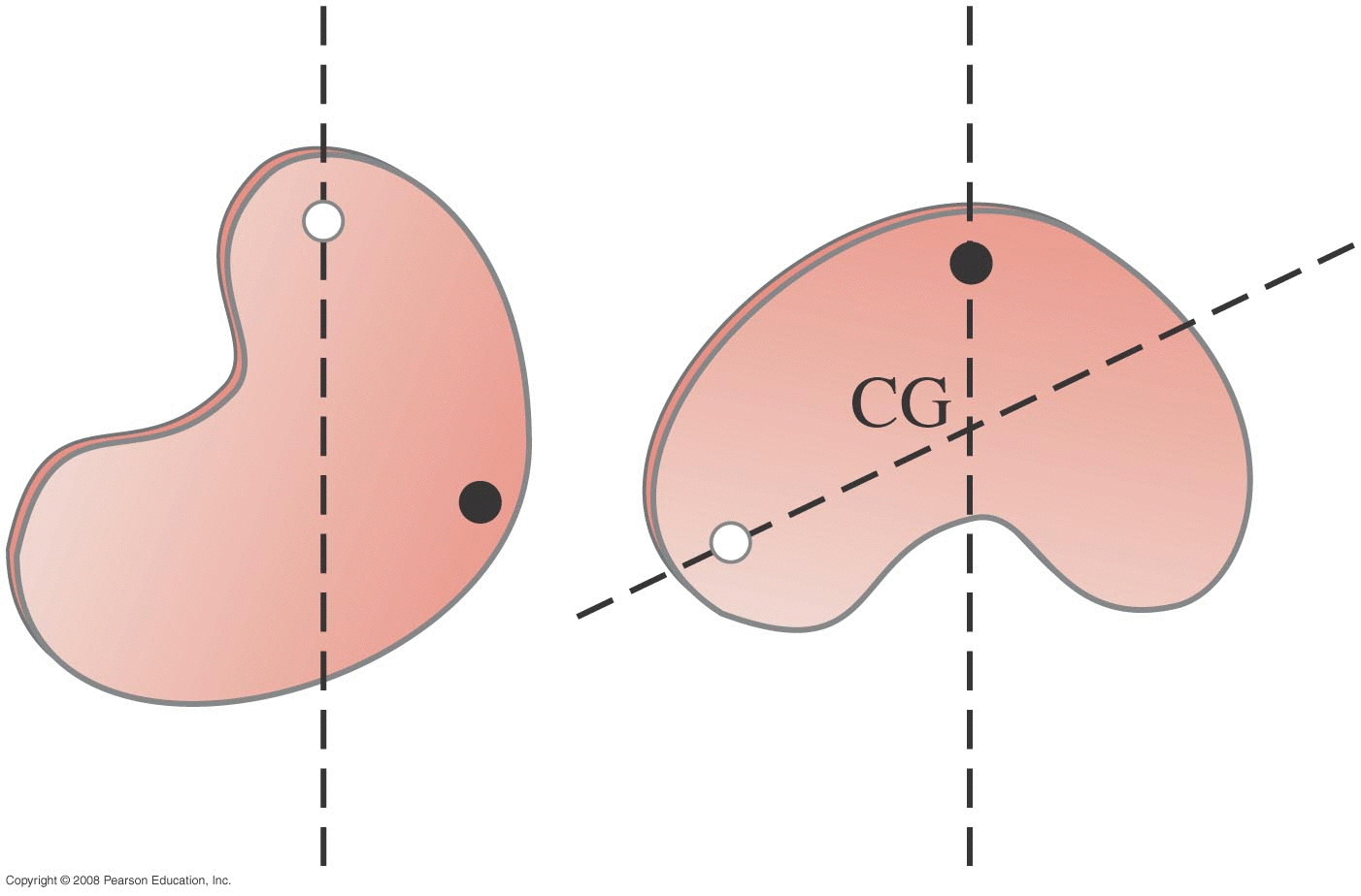
Suppose we have some object (like the baseball bat in this figure) that is constrained to rotate about some point (labelled O in the figure). The object will ultimately be rotating about point O, so let's attack this via rotational equations and concepts like torque. \[ \sum \vec{ \tau } = I \vec{ \alpha } \] Each external force acting on the object produces a torque of: \[ \vec{ \tau } = \vec{r} \times \vec{F} \] Recall that (vector) r is a vector that points from the axis of rotation to the point where the (vector) force F is being applied. 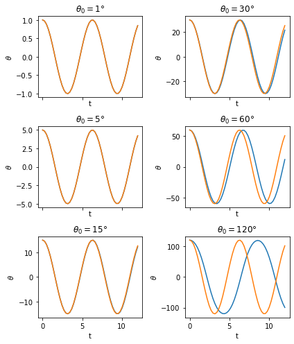What differential equation do we get this time? (One that we can't easily solve, unfortunately...)

Taylor Series Expansion of sine(x)

The Taylor Series expansion of the function sin(x) (with x in radians) is: \[ \sin{(x)} = x - \frac{x^3}{3!} + \frac{x^5}{5!} + \cdots \] The figure shows the actual sine(x) function compared to the Taylor Series expansion where we keep just the first term, and keeping the first two terms. The graph runs from 0 out to 90 degrees (π/2 radians). Most real pendulum scenarios involve pretty small angles, where even just keeping the first term sin(x)=x is 'good enough'.

So, IF our pendulum only swings back and forth to small angles, what does our DFQ turn into? One we can solve easily this time!   So what is the angular frequency ω and the period T for a physical pendulum (extended object)? a simple pendulum (point mass at the end of a massless rod)?

 

Simple vs Physical Pendulum
Let's consider the sort of pendulum in a grandfather clock.   First, assume a point mass at the end of a 1 meter long massless rod. What would the period of this pendulum be?   Next, assume the pendulum consists of a heavy flat disk whose CM is located exactly 1 meter from the axis of rotation. This time, we have a disk of 10 cm diameter with a mass of 4 kg, with the supporting rod still being massless.   Finally, what if the rod has a mass too? Suppose it extends all the way behind the disk to the 'other' edge, and has a mass of 0.2 kg. What would be the period of this pendulum?
The disk part of the pendulum has a knob that can be used to slide the disk up and down a bit. Why is that there?

 

'Exact' Simple Pendulum Solution

Technically the point-mass simple pendulum DFQ does have an exact solution, but it's in terms of an elliptic function which is expressed as an integral. It also just gives t(θ) for the first quarter-cycle only, which needs to be inverted to get θ(t) for that first quarter-cycle and then symmetry is used to generate the rest of the motion. So not particularly useful... The figure on the right compares the small-angle result (in orange) vs the exact solution (in blue) for various starting angles.

 

Practical (maybe) Value
For small oscillations, the period is related to the moment of inertia (about the rotation axis) and the distance to the CM of the object. \[ T_{physical} = 2 \pi \sqrt{ I / (mgh) } \] This provides a mechanism to determine the moment of inertia for oddball-shaped parts, by just letting them swing back and forth like a pendulum.
We'll need to find the CM but can do that using a trick from Chapter 9. Basically hang the object from some point. At the equilibrium position, the CM must be directly below that point. Do that for various points on the object and we can determine the exact CM.   Now letting the object oscillate back and forth, we know h (since we know where the CM is now) and we can measure the period T so that's enough to solve for I.   That will be the moment of inertia about the rotation axis, but we can use the parallel axis theorem to find the moment of inertia of the object for rotations about a parallel axis that passes through it's CM.   (These days, everything is done in CAD programs which can determine CM and I about various axes directly from the design of the part...)

 

Torsion Pendulum
Another type of oscillatory motion is a torsion pendulum in which some object (like the disk shown in the figure) is suspended by a wire. Twisting the object about that vertical axis will twist the wire, resulting in a 'linear restoring force' that's expressed as an angular force (i.e. a torque): \[ \tau = -\kappa\theta \hspace{2em} linear~restoring~torque \] Here then, Σ τ = I α yields the same DFQ we had with the mass on a spring and we can directly pick off the angular frequency of the motion: \[ \omega = \sqrt{\kappa/I} \] yielding a period of: \[ T = 2\pi \sqrt{I/\kappa} \] Doing this with a known object can be used to find the torsion constant κ of the wire (or beam, or ...). (NOTE: ME's define a very different quantity that they call the torsional constant, so don't confuse that with the definition used in our textbook.)
NOTE: if you watch the Tacoma Narrows bridge collapse videos, especially the longer ones, you'll see that the bridge is actually undergoing this 'torsional' motion leading up to the collapse. video     (Clear torsional oscillations around t=10 sec; t=2 min.)
Application: Cavendish Experiment
Around 1798, Henry Cavendish did an experiment that yielded the first good estimate for the universal gravitational constant G (the constant in the gravitational force equation: \[ F_g = G \frac{Mm}{r^2} \] (Actually he was more interested in finding the average density of the Earth and didn't bother to include the G value he found, but others later repeated the experiment focusing on estimating G.) In that experiment, the rod connecting the lighter metal balls (m) in the figure was suspended by a thin wire and then brought near the heavy fixed masses (M). The (incredibly tiny) gravitational force between the objects caused the lighter ones to move slightly, twisting the wire (a light shining on the mirror attached to the wire would make a spot that moved slightly on the wall so that the tiny angles could be measured).

 

14.7 : Damped Harmonic Motion
When we have a linear restoring force, we found that the object oscillates with the generic solution of \[ x(t) = A\cos{( \omega t + \phi ) } \] but that cosine would go on forever, and in the real world these oscillations usually (always?) diminish over time. In class, I held a meter-stick over the edge of the table and pulled up on the free end. When I let it go, that end vibrated up and down but and amplitude quickly died away.
One major reason is the presence of resistive forces like air resistance. For relatively slow motion, a good first approximation is: FR = -bv (force linearly proportional to the speed of the object through the medium).   Adding this force term to Newton's Laws: Σ F = ma becomes -kx-bv=ma or ma+bv+kx=0 and replacing a and v with the appropriate derivatives yields: \[ \frac{ d^2 x }{dt^2 } + (\frac{b}{m})\frac{dx}{dt} + (\frac{k}{m})x = 0 \]   The resistive force always does negative work, removing energy and slowing the object down, so we expect the period to be slightly different than before. The behavior 'looks like' a cosine that's exponentially decaying with time, so we'll guess a solution of: \[ x(t) = A e^{-\gamma t } \cos{ ( \omega' t ) } \] Doing so results in the exponential decay factor being: \[ \gamma = \frac{b}{2m} \] And the new frequency of the oscillation will be: \[ \omega^\prime = \sqrt{ \omega^2_o - \gamma^2 } \] where ωo is the undamped 'natural' frequency: \[ \omega_o = \sqrt{k/m} \]

 

Impact of Damping Factor
More damping (higher b) means larger γ (amplitude decays more quickly). Only up to a point though:   (A) underdamped (small 'b')   (B) critically damped ('b' is 'just right' to eliminate the oscillations entirely) (at this point ω'=0 so b=2mγ)   (C) overdamped : 'b' too large; object returns to equilibrium position very slowly   b>2mγ and ω' becomes imaginary(!)

 

Real-world Damping Scenarios
Shock Absorbers in Cars	Shock Absorbers in Buildings

 

Car Springs and Shock Absorbers
I looked up some numbers for actual cars and found one to use as an example. The car has a mass of M=1200 kg and each of the four springs has a spring constant of k=5000 N/m and a damping factor of b=545.5 N·s/m. We have four of these gadgets (one for each wheel), so in combination, the effective spring constant for this situation is k=20,000 N/m and the effective damping factor is b=2182 N·s/m.   Determine the undamped and damped periods of the motion of the car when it goes over a bump.
	Damped vs Un-damped Oscillations of the Car

 

14.8 : Forced Oscillations : Resonance
Here we'll add an extra external periodic (cosinusoidal) forcing function and look at the impact on the motion of the object.   \[ \frac{ d^2 x }{dt^2 } + (\frac{b}{m}) \frac{dx}{dt} + (\frac{k}{m})x = (\frac{F_o}{m}) \cos{(\omega t)} \]   where ω is the frequency of the forcing function (converted to f=ω/(2π) in the figure label)   The long term steady state solution will be of the form: \[ x(t) = A_o \sin{( \omega t + \phi ) } \] where: \[ A_o = \frac{ F_o }{ m \sqrt{ ( \omega^2 - \omega^2_o )^2 + b^2 \omega^2 / m^2 } } \]
Example: the previous car with shock absorbers drives over a road where the surface undulates cosinusoidally with an amplitude of 10 cm. The speed of the car will affect the 'frequency' of this 'forcing function'. How will the car behave as we change the frequency at which we pass over these bumps in the road?
Car amplitude as a function of (angular) frequency:	Car amplitude as a function of period (time between bumps):
I'll do an example in class with a mass hanging from a spring, then oscillate the top of the spring at various frequencies to illustrate this effect. If we 'force' the system at a frequency close to it's natural oscillation frequency, the amplitude of the oscillations can be quite large.
Real world examples: opera singers breaking glass, Tacoma Narrows bridge collapse, buildings in earthquakes, etc. Excellent video of sound breaking a wine glass in slow motion, showing the oscillations building up in the glass itself: video     (See around t=2 min and t=4 min)