15.3 : Energy/Power in P-Waves
Last time, we started with the energy in a little mass element as a wave passes through its location and found we could write: \[ E = 2 \pi^2 m f^2 A^2 \] and we used that to look at the energy and power in transverse waves on a linear medium like a wire or string. We can start from the same point and derive related expressions for energy and power for P-waves (longitudinal waves) in a gas or fluid (or solid, for that matter).
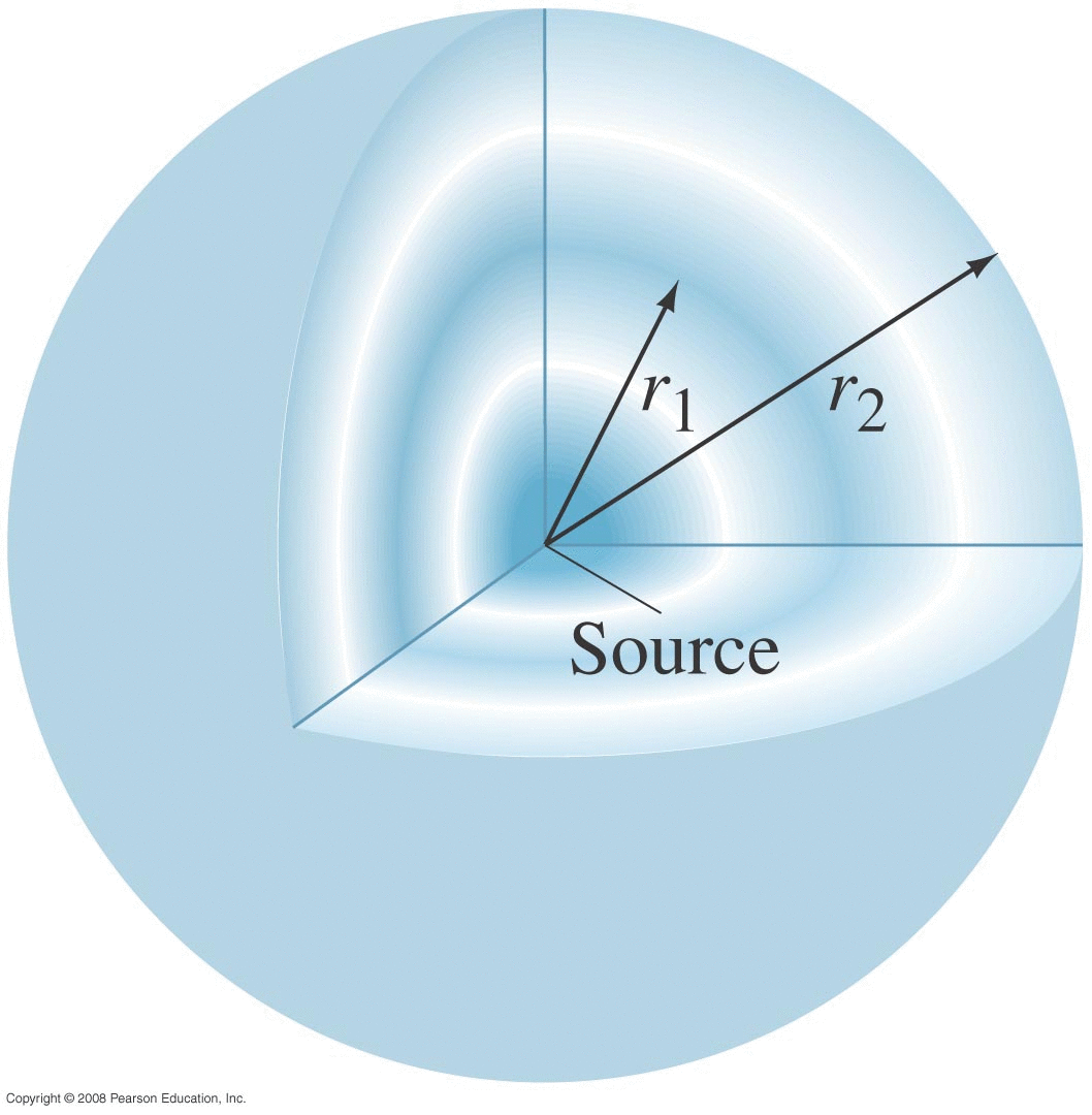
Source at origin with some power P
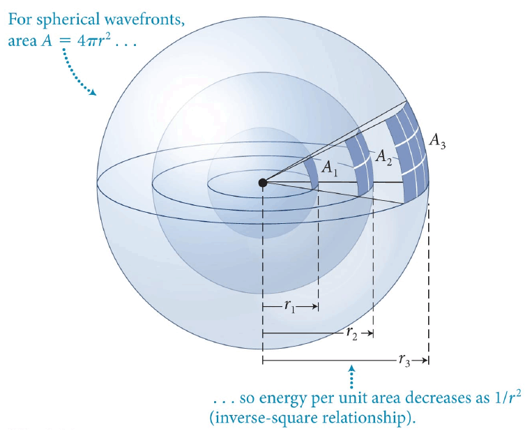
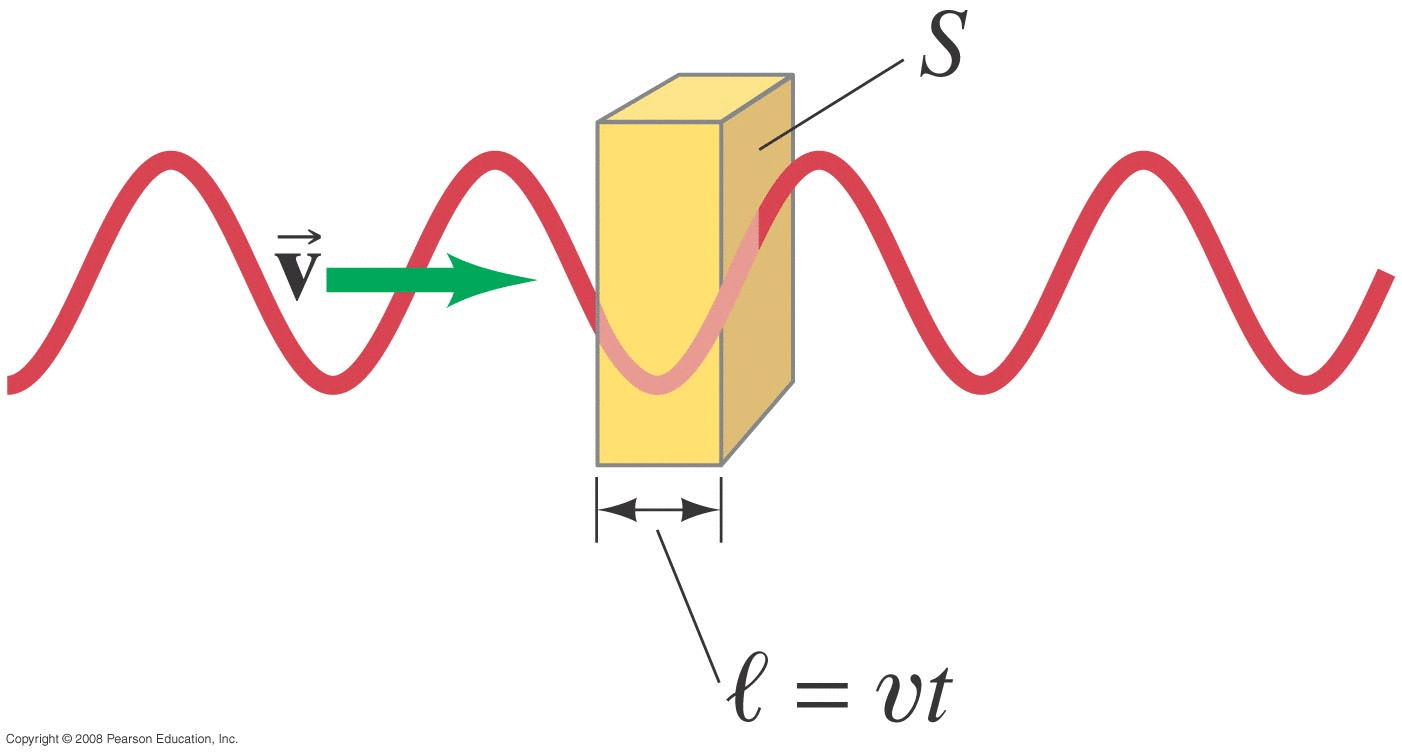
How much energy is present in a given volume (in particular the volume represented by how far the wave propagates in some time interval Δt. The mass involved now is the density times the volume: \[ m = (\rho)(S)(v\Delta t) \] so the energy (in joules) would be: \[ E = 2 \pi^2 \rho S v \Delta t f^2 A^2 \] Note: 'S' is the element area; 'A' is the wave amplitude
The power (energy per time) being carried by the wave then would be: \[ P = 2 \pi^2 \rho S v f^2 A^2 \] Related quantity: intensity is power per area (W/m2): \[ I = 2 \pi^2 \rho v f^2 A^2 \]
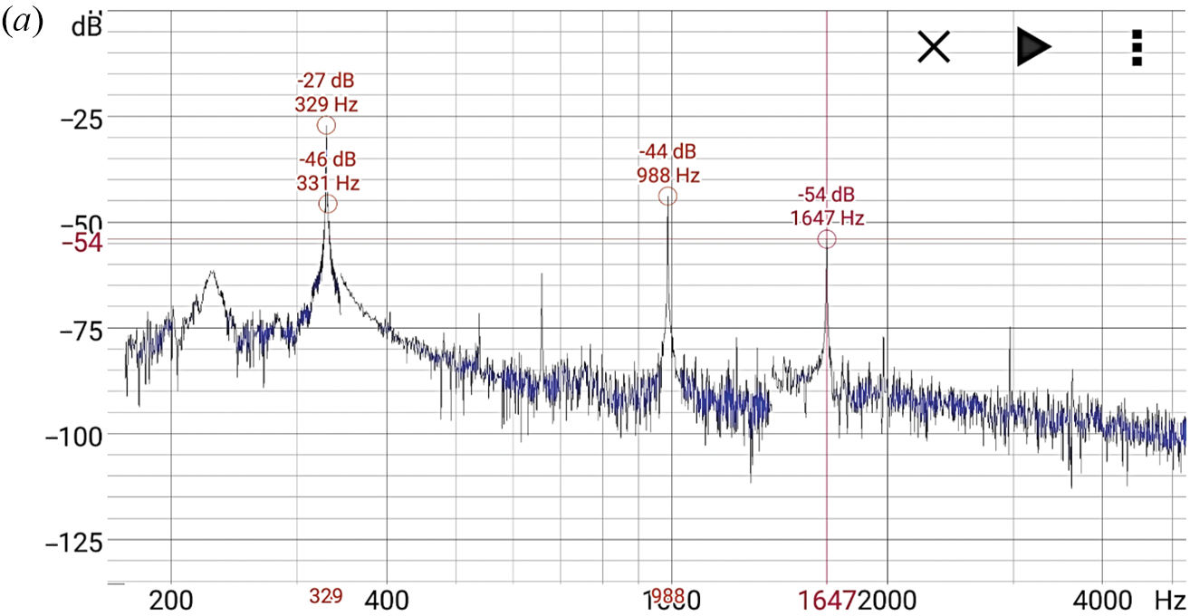
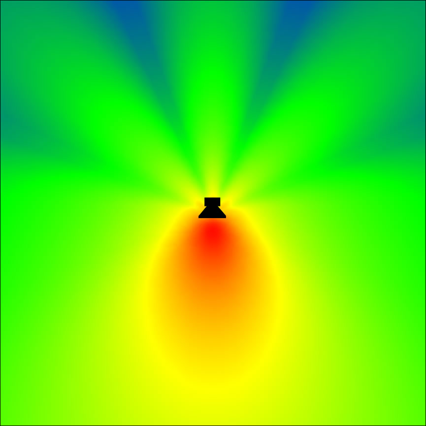
Example Suppose we have a 40 W speaker putting out a pure 1000 Hz tone. If we are 2 m away from the speaker, the air molecules are vibrating back and forth at what amplitude?   (Real speakers don't work this way, but assume the power is being uniformly radiated in all directions.)
Example : Back in the 60's when my family lived in Okinawa, an undersea volcano about 100 km away generated an earthquake that lasted about 2 minutes. In our neighborhood, I watched houses oscillate side to side with an amplitude of about A=10 cm with a frequency of about f = 0.1 Hz. (i.e. about 10 seconds between waves). For rock, v is (very) roughly 4500 m/s and ρ is (very) roughly 3000 kg/m3. Estimate how much power and energy was involved here? (Lots of assumptions here, so wouldn't be surprised if the actual values are 10 times higher or lower, but we should be vaguely close...)

 

f2 effect
Note that the energy, power and intensity all involve the square of the frequency. The higher the frequency, the harder it is to generate (the more power is required). Human hearing spans the range from 20 Hz to 20,000 Hz : a factor of 1000. If those waves had the same amplitude, the higher frequency would have (1000)2 times the intensity (loudness), and would cost the same factor as much power to generate. Lucky for us, most sounds we encounter (voice, music) have much lower amplitudes as the frequency increases. We still hear them clearly though since the power/intensity/loudness rises with frequency (squared).
Example: The graph at the right is a spectrum of the high-E string on a guitar. We'll see later what frequencies such a string should be generating, but for now note how the amplitudes drop off with frequency. The power is in decibels (a logarithmic scale; more later!). The main peak at 329 Hz represents about 50 times more power than the peak at 988 Hz, for example. Pure Notes: 329 Hz   988 Hz   1647 Hz   Actual high-E guitar string: (video)

 

1/r2 effect

Sound (and many other sources of waves) often send out waves in all directions, which means the source power is getting spread out over an ever expanding surface. Intensity is power per area: I=P/S=P/( 4πr2) Note that I is proportional to 1/r2 so if we want to compare the intensity (basically what our ear responds to) at one distance so the intensity at a different distance: \[ \frac{ I_2 }{I_1 } = \frac{ r^2_1 }{r^2_2 } \] Doubling the distance reduces the intensity (loudness) by a factor of 22 or 4. Halving the distance would increase the intensity (loudness) by a factor of 4.

 

15.5 : The Wave Equation
We started off with masses on springs, which lead to a simple second-order linear DFQ whose solutions we could write as simple sines and cosines. What equation yields travelling waves? \[ \frac{ \partial^2 D }{ \partial t^2 } = v^2 \frac{ \partial^2 D }{ \partial x^2 } \]   The textbook derives this for transverse waves on a string, which I won't duplicate here. We'll just show that our D(x,t)=A sin( kx-ωt ) form does satisfy the equation and move on to some of the implications of the wave equation that lead ultimately to how stringed instruments work.
The reason we mention all this here is that this equation appears in many scenarios that don't directly appear to involve waves. It appears in chemistry, crystal growth, fungus and bacteria growth, predator/prey models in biology, and many other scenarios. What it implies is that if the analysis of some scenario ends up yielding a differential equation that looks like the wave equation, then wave-like behavior will appear. Just like if the analysis of some scenario yields an equation that looks like d2 f / dt2 = -(constant) f then periodic (oscillatory) behavior will appear.
Chemical Waves : Belousov-Zhabotinsky Reaction
short video long video (with explanation; start 8:00) long video (with explanation; start 3:30)

 

15.6 : Principal of Superposition
The wave equation is linear which means that if D1(x,t) is a solution (maybe a sine wave travelling to the right) and D2(x,t) is another solution (maybe a Gaussian pulse travelling to the left), then any linear combination like D1+D2 is also a solution.
In the top figure, the three sine waves combine to create the shape just below them, so that shape propagating is really made up of the three sine waves all propagating together.                               In this set of figures, we see a collection of cosines or phase-shifted sines being used to try and build a square wave. Again, each sine or cosine will propagate through the medium with the same speed v, so the shape we built from them will maintain that shape and propagate along with that same speed v.     We've already talked about Fourier series - building almost arbitrary shapes from sines and cosines and here we're letting those waves propagate, retaining that arbitrary shape we started with.

 

15.7 : Reflection and Transmission
We'll see more on this later, but what happens to a wave that's travelling down a string (or any medium really) that is of finite length (i.e. a real string). Eventually we reach the end of the string (or other medium). What happens there? It strongly depends on the type of medium involved, but in the case of a transverse wave on a string, then:
• LEFT : If the end of the string is locked in place and can't move, the wave shape reflects but with an inverted amplitude. A positive amplitude (representing a displacement in one direction relative to the string) becomes a negative amplitude (a displacement in the opposite direction) when the pulse `reflects' from the end.   • RIGHT : If the end of the string is free to move, the pulse deflects that end of the string and reflects with the same sign
Video illustrating reflection: also interference
What if the string is connected to another string with a different mass/length (μ)? Maybe a string connected to a metal wire? The tension will be the same in each part of the medium but if μ is different then the wave speed \( v=\sqrt{F_t/\mu} \) will be different. In this figure a light rope is connected to a heavy rope (the higher μ will mean a slower v for the wave). In this case, part of the wave reflects (and flips sign) and part continues into the new medium (but with a different amplitude and wave speed). (We won't go into this now, but the fraction transmitted vs reflected depends on what's called the impedance of the material, which is basically the product of the wave speed on that material times it's mass/length μ.)

 

15.8 : Interference

The wave equation tells us that multiple waves can be present in a medium simultaneously and they all behave independently of each other. In the left figure below, we have a positive pulse travelling to the right and a negative pulse travelling to the left. They pass through one another. At one point they appear to have cancelled each other out, but at that point the string may have 0 displacement but the (tranverse) velocity and acceleration along the string isn't zero. In the right figure, we see how the two pulses (both positive this time) combine to create an extra high amplitude the instant they're both passing through the same point. (This is a mechanism for the rogue waves that sometimes make the news, where multiple wave fields combine to create a wave with exceptional amplitude.)     DIGRESSION: This effect can cause unexpected behavior in structures. If one component of a structure fails, a statics analysis might show that the new configuration is still stable (all the tensions and stresses will be different, but still may be within the tolerances of the components creating the structure). The problem is that the failure actually produces waves of changes in tension that are propagating through the structure, and these waves can constructively interfere with one another and yield much higher displacements (and hence tensions) briefly. Statics programs can't do these simulations so won't be able to alert the user to the possibility of this type of failure in the structure.

 

15.9 : Standing Waves : Resonance
The wave equation is linear, so suppose we have two identical waves (same amplitude, wavelength and frequency) travelling in opposite directions through some medium: Wave travelling in +X direction: D1(x,t) = A sin(kx - ωt) Wave travelling in -X direction: D2(x,t) = A sin(kx + ωt) The complete wave then would be: D = D1 + D2 = A [ sin(kx-ωt) + sin(kx+ωt) ] Recall from trig: sin(x±y)=sin(x)cos(y)±cos(x)sin(y) Expanding out those sines and combining terms, we end up with: \[ D(x,t) = 2A\sin{(kx)}\cos{ (\omega t) } \]
RIGHT : A plot of the situation above, called a standing wave since the nodal points don't actually move. There are actually two travelling waves present here, one going left and one going right, but the only actual motion we see is the up and down motion of the anti-nodes. The nodes will be located where the argument of the sine function is any integer multiple of π, : kx=Nπ. k=2π/λ so rearranging: x=N (λ/2)   that is: The nodes are located exactly a half-wavelength apart
Since the nodes don't propagate, if the medium is locked down at two such points (like the ends of a string in a guitar/piano/violin/..., the result is a pattern that oscillates up and down in place.   Here's a short video illustrating standing waves   The nodes are separated by λ/2, so for this to occur, the length of the string/wire/etc must be an integer multiple of λ/2: \[ L = N ( \frac{ \lambda }{2} ) \] We'll show that this implies the frequency of these oscillations will be: \[ f_N = N (\frac{v}{2L}) \] where v is the wave speed on the wire: \[ v = \sqrt{ F_T / \mu } \]
Example : On an 88-key piano, key number 28 plays a C note with a frequency of f=130.813 Hz. Suppose this wire has a length of L=1.10 m and a mass of M=9.00 grams. How much tension must this string be under in order to produce this frequency as it's fundamental? According to google search, should be about 944 N or 212 pounds. The total tension of a grand piano's wires is about 18 to 20 tons What other frequencies will this string vibrate at? Video of a violin string being played, showing various modes initially, but settling down to just the fundamental: violin string
Stringed Instruments : options for producing each note \[ f_1 = \frac{v}{2L} \] \[ v = \sqrt{ F_T / \mu } \] \[ \mu = M/L \] Combining those, ultimately: \[ f_1 = \frac{1}{2} \sqrt{ \frac{F_T}{ML} } \]
On a standard 88-key piano: the lowest key creates a frequency of f=27.5 Hz. the highest key creates a frequency of f=4186 Hz. That's a range of a factor of about 152.2, which means that the blob under the square-root must be able to vary by a factor of (152.2)2 or 23,170.   How is that achieved? different tensions (only a factor of 2 here) length varies from 2 meters to 5 cm (factor of 40) string thickness varies from 0.79 mm to 6.1 mm (mass ∝ volume ∝ r2, so a factor of 60 here) different materials (guitars, bass) added mass (wire-wrapped: piano, guitar, ...)   Guitars, violins, etc have it much easier : much smaller frequency range, so all the strings are typically the same length and the different frequencies can be created by altering the tension of each string, and/or making them from different materials.

 

Normal Mode Naming Conventions
We'll see more of this in the next chapter, but these normal modes have two naming conventions attached to them:   Fundamental and Overtones vs Harmonics
Guitar String Revisited
Recall the spectrum of a vibrating high-E guitar string from before. We see peaks at: f1=329 Hz f3=988 Hz f5=1647 Hz Why is the spectrum dominated by just the ODD N modes?

When you 'pluck' a string, you displace the string laterally. Various sine waves are needed to create that shape, and those then propagate back and force on the string, with the various harmonics being the only patterns that 'survive' and continue to resonate. Where you pluck the string changes that initial displacement, and what sines are needed to create that shape.   In the figures below, the same guitar string (the 'A' note on a Fender Bass guitar) is plucked at two locations:
Plucked at the 'usual' location (over the pickups) Note that the N=1 (fundamental) is fairly weak; the N=2 and N=3 modes are much stronger (so apparently very little of the N=1 'sine shape' was needed here).	Plucked near the center of the string In this case, all the modes seem to be present (unlike in the acoustic guitar spectrum earlier), with quite a few modes of similar strength needed to represent the initial displacement.
Normal Modes in Other Objects
A baseball bat : video (actual) Wood vs Metal bats : video (animations) An empty beer bottle : video (animations) Drum head : video