Chapter 37 : Early Quantum Theory and Models of the Atom

Problem : Black-body Spectrum

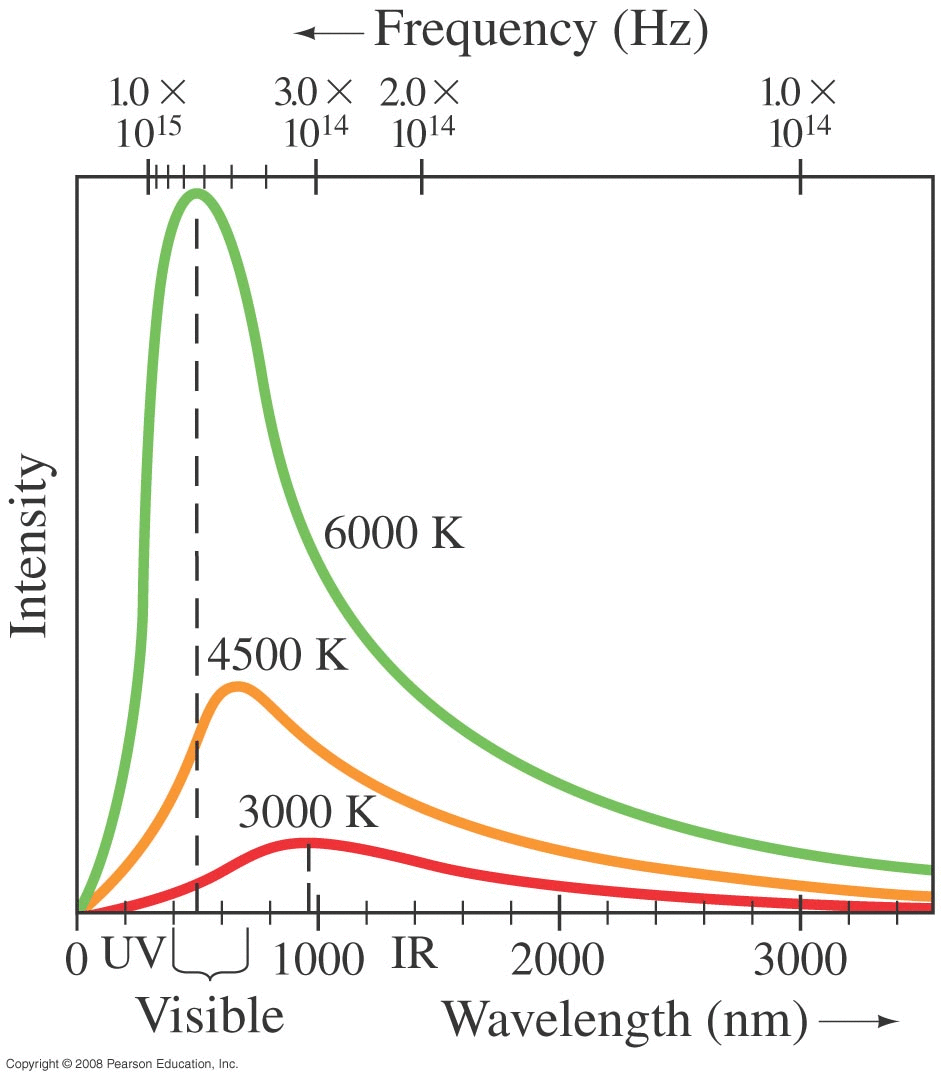
When a sample is heated up, it radiates energy in a predictable way, called black-body radiation yielding an intensity spectrum like those shown here.
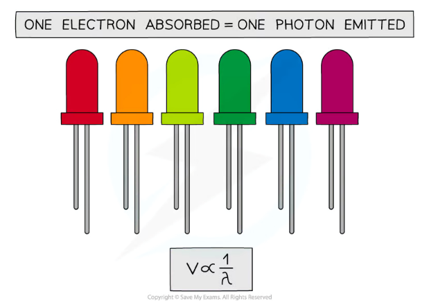
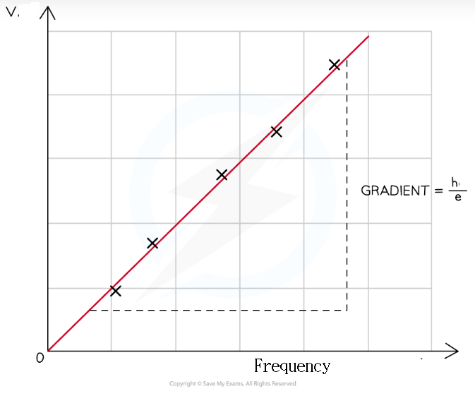
Circa 1900, Max Planck borrowed ideas from thermodynamics (basically statistics of huge numbers of particles) and showed heat would behave the same way if treated as a vast number of (massless) entities called photons, each carrying an energy of:
\[ E = hf = hc/\lambda \]

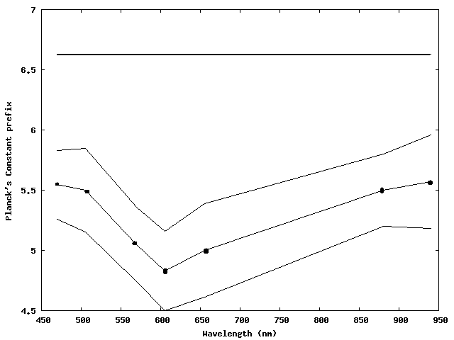
where h=6.6261 X 10^-34 J·s
(now called Planck's constant)

The resulting intensity spectrum was:
\[ I(\lambda,T) = \frac{ 2 \pi h c^2 \lambda^{-5} }{ e^{hc/(\lambda kT)} - 1 } \]

(Note: here k isn't the Coulomb constant, but the Boltzmann constant that appears in thermodynamics.)

Examples :

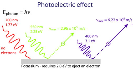
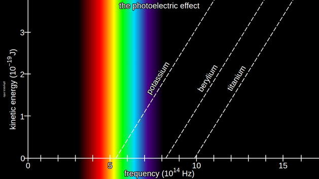
How much energy would a 'photon' of visible light carry?

Violet: λ=390 nm = [what] in Joules? In electron volts?
Red: λ=750 nm = [what] in Joules? In electron volts?

X-ray photons : energies from 100 eV to 100 keV
Gamma rays : in the MeV range
Most energetic photon ever detected: 18 TeV

Problem : Atomic Spectra

Not all materials emit continuous spectra.

When current passes through a gas (or any material vaporized into a gas or plasma), the resulting spectrum only had very specific frequencies.

Gas discharge tube
(schematic)

Gas discharge tube
(actual)

Spectrum of hydrogen

Spectrum of helium

Spectrum of iron

Geissler Tubes (1860's)

Problem : Photoelectric Effect

From PH2223 : the electroscope was a device used to experiment with electricity in the mid 1800's. Charges transferred to the top plate would cause the 'leaves' of the electroscope to swing apart.

It was found that just shining light (in particular ultraviolet light) on the device would cause the leaves to separate.
Worse still:

As the wavelength increased, the effect diminished, eventually disappearing altogether, no matter how intense the light was.
Different metals responded to different frequency ranges.

Electroscope (1869)

The electron had been discovered in 1897.
Here is the result of an actual experiment from 1916 using metallic sodium as the target.
Light of various wavelengths was aimed at the target and the kinetic energy of the ejected electrons was measured (by measuring the voltage needed to stop them).
Below a frequency corresponding to λ=683 nm (red) no current resulted.

The model here is the incoming photon has some energy E which goes first into breaking the electron free from the metal (an amount called the work function of the material), then whatever was left went into the KE of the electron.

Measuring h Using the Photoelectric Effect

\[ E_\gamma = hf = W + K \]

At the 'stopping voltage', K = e V_s so:
\[ hf = W + eV_s \]
or:
\[ V_s = ( \frac{h}{e} ) f - (\frac{1}{e})W \]

The slope of the stopping-voltage needed vs the frequency of the incoming light would be h/e and the charge on the electron was known, so this experiment would yield a value for h

The experiment can be done with various materials, all of which have different work functions, but the slopes will all be the same: h/e.

Measuring h Using an LED (next lab)

This process is slightly different from above.
In the lab, you'll gradually increase the voltage applied to a light-emitting diode (LED).
When this voltage is high enough, the energy given to the electron: E=(e)(V) is enough to cause it to escape from an atom; when it is recaptured by an atom it releases that energy in the form of a photon with energy E=hf.
implies: eV=hf or V=hf/e
Plotting this threshhold voltage vs the frequency of the light emitted, the line should have a slope of (h/e)

Last year's result:

The lab has you plot the voltage vs the LED frequency (f=c/λ) and find the slope, which should be (h/e).
Since the 'intercept' here is zero, we can also use each single measurement to estimate h=(e)(V)(λ)/c
This graph does that calculation for each wavelength, using the data from all the lab reports.
The result is an estimate for h that was about 20 percent below the actual value.

Please send me a copy of your lab report (in particular the voltage values for each color LED you use) so I can update this graph.

Problem: Rutherford Experiment

Done in the late 1890's.
Alpha particles from radioactive radium or uranium were pass through a very thin gold foil.
If matter was continuous, the particles would spread as they passed through the material.
Instead, the vast majority of the particles went straight through.
A few were deflected, in some cases nearly straight back.

Apparently the atom was mostly empty space:

Approximate dimensions implied by the experiment:

Bohr Model of the Atom (1913)

This is the classic high school model of an atom: a tiny positively charged nucleus being orbitted by negatively charged electrons.

Let's assume we have Z positive charges (protons) in the nucleus, but just one single electron in orbit.

F=ma with the radially-inward Coulomb force:
\[ \frac{1}{4\pi \epsilon_o}Ze^2/r^2 = mv^2/r \]

What would the kinetic energy of the electron be: K(r)=?
What would the electric potential energy of the electron be U(r)=?
What then is the total mechanical energy of the electron E(r)=?

Photoelectric effect explained: the electron is 'bound' to the atom. Some minimum energy is needed to overcome its (negative) E in order to be released.
Spectra sort-of explained: an electron moving from one radius to another involves gaining or releasing energy

New problem though: r could be anything, so photons of any energy (wavelength) should still be present. Why aren't they?

By looking at the actual wavelengths emitted by hydrogen, Bohr found that they could be explained IF the electron could only be at certain specific r values which happened to be where their angular momentum was L = n(h/2π) for n=1,2,3,...
That is, their angular momentum was QUANTIZED.

Angular Momentum

Recall, angular momentum is the rotational variant of linear momentum (p=mv), that is L=Iω
For a point mass: I=mr² so L=(mr²)ω=(mr²)(r/ω)=mvr

Quantized Angular Momentum: Impact on Real-World Scales

Consider a golf-ball rotating with a frequency of about f=2 Hz.
What angular momentum does that represent?
As the golf ball slows down, it has to jump from one L to the next 'allowed' value for L.
How many h/(2π) units is that?
Can we `see' this happening?

Solid sphere: I=⅖MR²
Golf ball

M = 46 grams = 0.046 kg
R = 2.134 cm = 0.02134 m
I = ⅖MR² = 8.4 X 10^-6 kg m²
ω=2πf=12.6 s^-1
L = Iω = 1 X 10^{-4} kg m² s^-1
Fundamental unit of angular momentum: h/(2π) = 1.055 X 10^-34 J s
Works out to n=9.5 X 10²⁹

The golf ball doesn't uniformly slow down to a stop, it takes about 10³⁰ steps to do so. (Impossible to measure!)

This effect can be ignored until we get down to molecular/atomic scales, which folks in the nanotechnology area are dealing with...

Bohr Model : 'Allowed' Energy Levels

(a) F=ma (radial) with F_E:
\[ k \frac{(Ze)(e)}{r^2} = m \frac{ v^2 }{r} \]

(b) Rearrange to solve for r:
\[ r = \frac{ k Z e^2 }{mv^2} \]

(c) The angular momentum of the electron must be quantized:
\[ L = mvr = n \frac{h}{2\pi} \]

(d) Rearrange:
\[ v = \frac{nh}{2 \pi m r } \]

(e) Replace 'v' in (b) with this and rearrange:
\[ r_n = \frac{ n^2 h^2 \epsilon_o }{\pi m Z e^2 } \]

(f) Or more compactly:
\[ r_n = \frac{ n^2 }{Z} r_1 \]

where r₁, called the Bohr radius is:
\[ r_1 = \frac{ h^2 \epsilon_o }{\pi m e^2 } \]

For a hydrogen atom, n=1 and Z=1 so: r₁ = 0.529 X 10^-10 m.
The diameter of a single hydrogen atom should be about 0.1 nm.

Atomic Radii

Substituting this expression for r into our equation for the electron's total energy at a given radius, the energy levels are restricted to these values:
\[ E_n = -( \frac{ Z^2 e^4 m }{ 8 \epsilon^2_o h^2 } ) \frac{1}{n^2} \]

We're dealing with such small energies, judicious units conversions lead to:
\[ E_n = -(13.6~eV) \frac{Z^2}{n^2} \]

The electron MUST be in one of these 'orbits'
An 'excited' electron can drop to a lower orbit, releasing that energy as a photon that has exactly that amount of ΔE, corresponding to a wavelength via E=hc/λ
An incoming photon of just the right energy can knock an electron into a higher orbit

Hydrogen Emission Spectrum

The Lyman series (electron dropping to n=1 from some higher orbit) represents energy changes from 13.6 eV to 10.2 eV and using E=(1240 eV nm)/λ this implies light wavelengths between 91 nm and 121 nm, meaning they're in the ultraviolet (not visible) range.
The Balmer series (electron dropping from some higher orbit to n=2) involves ΔE between 3.4 eV and 1.9 eV corresponding to wavelengths between 365 nm and 653 nm and most of those transitions create light in the visible range.
The Paschen series represents ΔE between 1.5 eV and 0.65 eV, corresponding to wavelengths between 827 nm and 1908 nm, which are in the infrared range.

Absorption and Emission in Nebulae

Problem : Atomic Spectra
Not all materials emit continuous spectra. When current passes through a gas (or any material vaporized into a gas or plasma), the resulting spectrum only had very specific frequencies.	Gas discharge tube (schematic)	Gas discharge tube (actual)
Spectrum of hydrogen
Spectrum of helium
Spectrum of iron
Geissler Tubes (1860's)

Problem : Photoelectric Effect
From PH2223 : the electroscope was a device used to experiment with electricity in the mid 1800's. Charges transferred to the top plate would cause the 'leaves' of the electroscope to swing apart. It was found that just shining light (in particular ultraviolet light) on the device would cause the leaves to separate. Worse still: As the wavelength increased, the effect diminished, eventually disappearing altogether, no matter how intense the light was. Different metals responded to different frequency ranges.	Electroscope (1869)
The electron had been discovered in 1897. Here is the result of an actual experiment from 1916 using metallic sodium as the target. Light of various wavelengths was aimed at the target and the kinetic energy of the ejected electrons was measured (by measuring the voltage needed to stop them). Below a frequency corresponding to λ=683 nm (red) no current resulted.
The model here is the incoming photon has some energy E which goes first into breaking the electron free from the metal (an amount called the work function of the material), then whatever was left went into the KE of the electron.

Bohr Model : 'Allowed' Energy Levels
(a) F=ma (radial) with F_E: \[ k \frac{(Ze)(e)}{r^2} = m \frac{ v^2 }{r} \] (b) Rearrange to solve for r: \[ r = \frac{ k Z e^2 }{mv^2} \] (c) The angular momentum of the electron must be quantized: \[ L = mvr = n \frac{h}{2\pi} \] (d) Rearrange: \[ v = \frac{nh}{2 \pi m r } \] (e) Replace 'v' in (b) with this and rearrange: \[ r_n = \frac{ n^2 h^2 \epsilon_o }{\pi m Z e^2 } \]
(f) Or more compactly: \[ r_n = \frac{ n^2 }{Z} r_1 \] where r₁, called the Bohr radius is: \[ r_1 = \frac{ h^2 \epsilon_o }{\pi m e^2 } \] For a hydrogen atom, n=1 and Z=1 so: r₁ = 0.529 X 10^-10 m. The diameter of a single hydrogen atom should be about 0.1 nm.
Atomic Radii

Substituting this expression for r into our equation for the electron's total energy at a given radius, the energy levels are restricted to these values: \[ E_n = -( \frac{ Z^2 e^4 m }{ 8 \epsilon^2_o h^2 } ) \frac{1}{n^2} \] We're dealing with such small energies, judicious units conversions lead to: \[ E_n = -(13.6~eV) \frac{Z^2}{n^2} \] The electron MUST be in one of these 'orbits' An 'excited' electron can drop to a lower orbit, releasing that energy as a photon that has exactly that amount of ΔE, corresponding to a wavelength via E=hc/λ An incoming photon of just the right energy can knock an electron into a higher orbit
Hydrogen Emission Spectrum The Lyman series (electron dropping to n=1 from some higher orbit) represents energy changes from 13.6 eV to 10.2 eV and using E=(1240 eV nm)/λ this implies light wavelengths between 91 nm and 121 nm, meaning they're in the ultraviolet (not visible) range. The Balmer series (electron dropping from some higher orbit to n=2) involves ΔE between 3.4 eV and 1.9 eV corresponding to wavelengths between 365 nm and 653 nm and most of those transitions create light in the visible range. The Paschen series represents ΔE between 1.5 eV and 0.65 eV, corresponding to wavelengths between 827 nm and 1908 nm, which are in the infrared range.